What's Priced In?
Stock prices are the clearest and most reliable signal of the market’s expectations for a business’s future performance. Ignore them at your peril!

Overview: The value of a business (or any cash-generating asset) is the present value of its future cash flows. If you knew the magnitude and timing of a business’s future cash flows as well as the appropriate rate at which to discount them, then you would know the precise value of the business.
Unfortunately, valuation isn’t that easy in the real world – with equities we know none of these variables with precision. Forecasts are prone to a myriad of problems. For example:
- Garbage-in, garbage-out: the accuracy of a forecast is only as good as the accuracy of the forecaster’s underlying assumptions.
- Standard DCF models usually have an explicit forecast period of 3-5 years, whereas the market discounts many years of future cash flows in calculating present value. There is a good argument for why analysts use such a short forecast horizon: any forecast beyond a couple of years is suspect. However, that leads to serious limitations in forecasting (fortunately, as we’ll see below, there is a way around this issue).
- Accurate forecasting requires knowledge of the appropriate reference class’s base rates, which is often difficult to ascertain.
- Most investors use the capital asset pricing model (CAPM) to determine the appropriate discount rate. However, the cost of equity, an input into the CAPM, has been proven to be a poor predictor of future share price movements.
- Forecasts can create anchoring bias in the forecaster, as well as overconfidence and confirmation bias. Many analysts “marry their model”.
- There are many other issues, but you get the point!
Using multiples as your chosen investing methodology has its own flaws – multiples are short-hand for the DCF process, however with multiples all the assumptions are hidden. At least with a DCF model the assumptions are explicit. Explicit assumptions can be debated and compared to base rates – with multiples we lose even that.
All in all, forecasts of future cash flows are rife with problems, and forecasts often tell you more about the forecaster than they do about the future (for exceptions to that, see Philip Tetlock's excellent book Superforecasters).
We can, however, invert the valuation process: using the current market valuation as a guide to what is priced into the stock.
Stock prices are the clearest and most reliable signal of the market’s expectations for a business’s future performance. The single point of price represents a distribution of outcomes that individual market participants expect to occur. Successful investing requires estimating the level of expected performance embedded in the current stock price and then assessing the likelihood of a future revision in expectations. Michael Mauboussin wrote a great book on this topic called Expectations Investing. It’s a must read.
Mauboussin’s methodology is one of six methods I use to estimate what is priced into a stock. Mauboussin’s methodology can be enhanced by going beyond consensus revenue and margin estimates and asking, “what unit economics does this imply”? The goal is to back into the implied unit economics of a business rather than just the implied high-level financials. More specifically, the goal is to find gaps between implied future unit economics and actual future unit economics. I address this topic in depth in another post, unit economics and cohort retention curves.
“All models are wrong, but some are useful.” John Maynard Keynes said “I’d rather be vaguely right than precisely wrong”. Let’s take these simple concepts seriously.
Each method has its own strengths and weaknesses. They are all based upon the conceptual framework of a DCF model. The methods are as follows:
- Reverse Hurdler (RH)
- Modified-Mauboussin-Method (MMM)
- Abbreviated-Mauboussin-Method (AMM)
- Reverse Modigliani & Miller Model (RMMM)
- Three-Staged P.I.E. (TSP)
- Gap Between Implied & Observation (GBIO)
Let’s walk through each of these methods below for the NYT. The order of the methods is important in terms of your return-on-time.
1: Reverse Hurdler (RH)
Valuation shortcut example for NYT:
The NYT's EV is ~$8bn (as of 2020.12.11). For this to be a 30% IRR (using 30% as an illustrative example of one’s hurdle rate) over ten years, that implies an exit EV of $110bn in 2030. What would it take to achieve this?
- Let’s assume a 40% NOPLAT margin in 2031 (we can debate this & alter it for other companies etc/do a sensitivity analysis), and that it trades at 15x forward NOPLAT (again we can use a sensitivity analysis). This implies a 6x forward revenue multiple.
- This valuation would require the NYT to generate ~$18bn in revenue in 2031, up from ~$2bn in 2021E (however print circulation is likely to stay flat/decline after accounting for pricing power, and print advertising will decline substantially. Print is largely bundled with digital today.)
- Assuming $750m in revenue from print (physical subscriptions/copies + advertising), that means just over $17bn in digital revenue.
- So the question becomes, can digital revenue get to $17bn by 2031?
- If digital revenue is split 80/20 between subscription revenue and advertising, respectively (again, up for debate/further research), that means ~$13.6bn in subscription revenue.
- What would it take to have $13.6bn in subscription revenues in terms of number of users & ARPU?
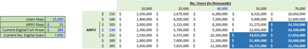
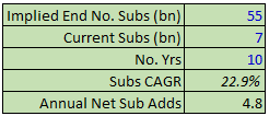
We can see from here that to get to a 30% IRR the Times needs to reach at least 55m subscribers, up from 7m today. Over 10 years that implies a 23% subscriber growth CAGR & an average of 4.8m net new subscriber adds per year:
Subscriber growth has been faster than that since the NYT introduced its subscription product in 2011. However, even in 2020 the Times has ‘only’ added 2m subs. Is it realistic that the business can add more than double that each year over the next ten years? Personally I think that’s pushing it and that one shouldn’t expect a 30% IRR from the stock.
Re-doing this analysis for a 20% IRR hurdle would require NYT reaching $8.3bn in revenue by 2031, or ~$7.5bn in digital revenue of which if 80% is from subscription revenue then $6bn in subscription revenue is required. Looking at this same sensitivity table, getting to 25m subs or more is required, which would be a 13.6% CAGR in number of users, or ~1.8m sub additions each year. This appears more reasonable, and so if one’s hurdle rate is 20% I’d suggest digging into the NYT. If your hurdle rate is 30% you likely have to believe in higher long-term margins (which is possible in the digital realm) or share buybacks/dividends/asset sales/new product launches hopping you across the 30% finish line.
The strengths of the RH include:
- It takes a bottoms-up perspective. Most analysis starts from the top and frames the TAM based on population, paying sub penetration, ARPU, LT margins, etc to come to a view on what a business is worth. RH inverses the problem and says, “to earn 30% annually, that means this business has to be worth $xx in 10 years” and then work your way back to the key variable to see if that is feasible.
- This is why I do this analysis first before any of the other methodologies. I’d rather spend time on something that has the potential to be a 30% IRR than on something that is clearly never going to be a 30% IRR.
The weaknesses of the RH include:
- You must compare your views on what’s “reasonable” to what’s priced in. Clearly, this is subjective since the future is unknowable in the present. If your views are way off on what’s “reasonable”, then this analysis won’t help you at all. That may be caused by a lack of understanding about the business, but it could also be caused by the competitive landscape evolving in a way that no one (or few people, at least) could have predicted.
- Many investors scoff at the idea of ignoring the CAPM when determining the appropriate discount rate to use. This is due to people considering the cost of capital to be the average market participant’s cost of capital. The reality is that different market participants have different opportunity costs & objectives. Insurance companies and pension funds need to match their liabilities, and are often happy to accept a 6% rate of return. Personally I want to generate much higher returns than that and I have a much higher risk tolerance than the average investor. Accordingly my opportunity cost & thus discount rate should be higher, too.
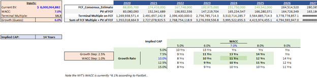
2: Modified-Mauboussin-Method (MMM)
Here I do use the CAPM to derive a stock’s WACC rather than just using my hurdle rate, because I’m trying to see what other investors are explicitly modeling. The goal of this analysis is to see exactly how market participants think about the company in question, not to see if it meets an IRR hurdle.
For the NYT specifically we’re able to get the implied unit economics including churn and return on advertising spend by inspecting the NYT’s historical financials as well as knowing the digital product’s price points and the starting and ending number of subscribers. I’ll post a video showing how to do this in the near future.
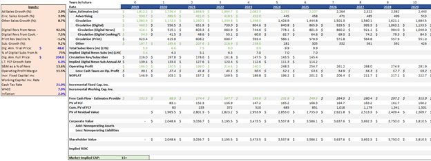
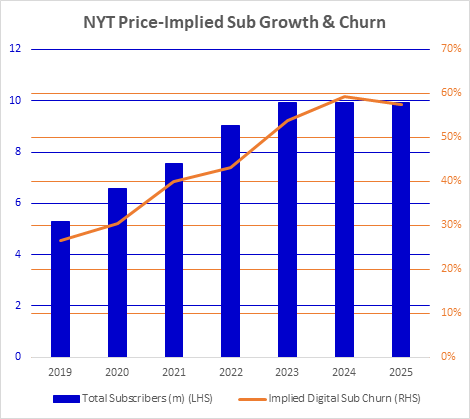
Using this method we can see some interesting things – for one, the market is implying that the NYT’s churn in the future will increase from its historical figures:
The strengths of the MMM are:
- It shows analyst consensus and ranges, so we can see what high level financials are explicitly being priced in.
- You can see what Competitive Advantage Period is being priced in.
- Depending on the business model and the complexity of the business, we can see what unit economics are being priced in, too. For the NYT we can see implied churn doubles from actual of ~30% in 2019 to 60% in 2025, which would be a dramatic decrease in retention. Alternatively the market could be saying that ROAS will decrease dramatically in the future, or some combination of increasing churn and declining ROAS. Given the company’s massive economies of scale in content creation as well as their brand, this seems unlikely to occur.
The weaknesses of MMM are:
- Not every business has many sell-side analysts working on it, so consensus estimates can be way off from what the market thinks. Even if a business has thirty sell-side analysts working on it, those thirty figures still only represent the consensus of those thirty analysts, not of the market itself.
- Consensus estimates only show you a few years out. Sometimes in Year 5 the estimate will only be from one analyst when there were 10 analysts in the 3-year forecast. This can cause strange jumps in consensus figures.
- Consensus estimates can have addition issues – e.g. if there are three analysts each with different forecasts on margin structure, the average revenue figure and the average FCF generation may not seem to add up.
3: Abbreviated Mauboussin Method (AMM)
We can shortcut Mauboussin’s method and just look at the free cash flow to see what the implied CAP is. This is useful if you want to quickly see how strong the market deems the business’s competitive advantage to be:
The downside to the AMM is that this method optimizes for expediency over transparency (we can’t back into implied margins etc looking only FCF…) But it is an expedient way to see the implied CAP and gauge what the market thinks about the business quality & durability.
4: Reverse Modigliani & Miller Model (RMMM)
Modigliani & Miller came up with a simple formula to split the value of a business into two components: the steady-state-value and the present value of future growth opportunities. The formula is simple:
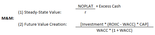
Applying this formula to the NYT (and making some assumptions around 2021 Investment as well as WACC and CAP):
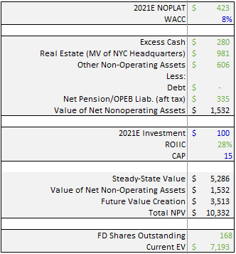
These assumptions should be sensitized, but we can see using these assumptions that the estimated value of the enterprise today is $10.3bn vs current EV of $7.2bn.
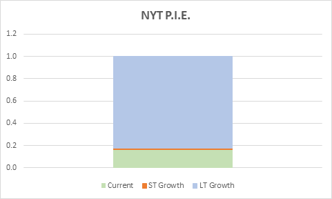
5: Three-Staged P.I.E. (TSP)
Here we take the M&M model one stage further by breaking down present value into three components: zero growth value (equivalent to Steady-State Value above); Value Creation from ST Growth (net of Zero Growth Value); and Implied Value Creation from LT Growth, which is a plug based on the current EV and the two aforementioned pieces. We can visualize this split using either a pie chart or a stacked bar (issues with pie charts arise when one of the values is negative).
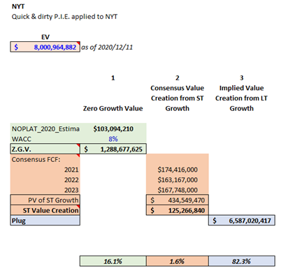
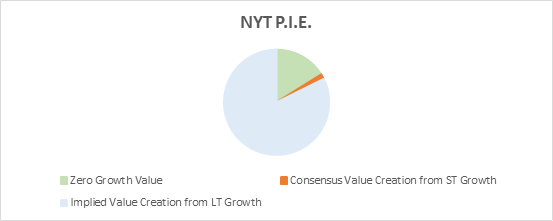
The strengths of TSP are:
- It’s fast & easy to do. As long as you have consensus estimates you only need to make one explicit forecast i.e. what growth will be after the explicit forecast period.
- It helps you visualize what the market is pricing in easier than any of the other methods. You can see when the value creation is expected to occur.
The weaknesses of TSP include:
- Often the first four years capture a very tiny percent of the overall value.
- It doesn’t show you detail on unit economics or even high level financials like revenue and margins.
- It also doesn’t show you if the business meets your hurdle rate.
6: Gap Between Implied & Observation (GBIO)
It is better to observe than it is to predict. In that vain, another simple model is to look at implied future growth vs observed historical growth:
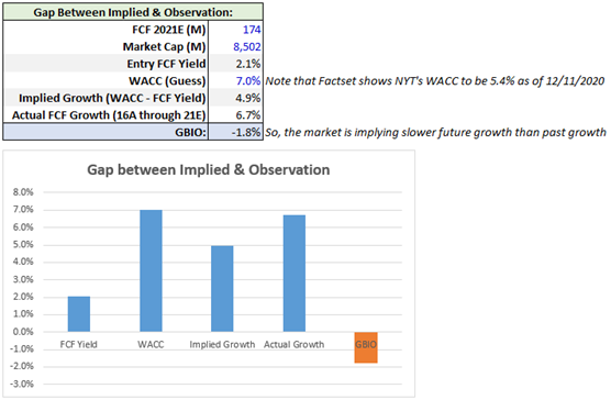
We can see that the market expects future FCF growth to decelerate vs what the NYT has achieved over the past five years (by 1.8% annually). Given the superior economics of digital subscriptions and the fact that growth in digital subscriptions is likely to cause overall growth to accelerate, a deceleration in FCF growth at the NYT seems unlikely in the near future.
Summary:
Inverting the valuation process enables investors to avoid many of the pitfalls of forecasting. It is helpful as a tool to see quickly whether something is worth digging into or not, based upon the gap between what’s implied and what one can observe historically as well as one’s views on the future of an industry/a business.